About

Authors

XML Format

Decision Support Shell on Web

Screenshots

Decision Support Shell on Palm

Spotlight

A paper on LogReg is available (both paper and presentation are avaiable in Slovene as well).

A PowerPoint presentation on decisions at hand concept is available.

FRI > Biolab > Decisions at Hand > Decision Support Scheme

Decision Support Scheme

Decision Support Scheme, in this document also referred to DSScheme or simply as scheme, is an XML document that encodes a particular decision model or particular set of decision models and participating variables. The DSScheme defines:

A textual description of the scheme, including names of authors, date of publishing and scheme's title.
List of variables that participate in the scheme. This includes names and IDs, variable types, and presentation format. We refer to variables in this list as "original variables". Original variables are those that user sees in the input window of particular application that uses DSScheme. Variables can be arranged in "slots" or pages, and if this is so, an ID of a particular page is associated with a variable.
List of pages that are used by DSScheme. Typically, if a DSScheme is used through a web-based interface, different pages of variables would still appear on the same input web page, but variables belonging to the same "page" would be grouped (page by page), and groups of variables would be separated by some divider (e.g., horizontal rule). On PDA's, due to physical limits of display, an input screen would indeed be organized page-by-page, potentially using different panes.
List of variables that are derived from original variables or from previously defined derived variables through some form of transformation (e.g., categorization, algebraic manipulation, etc.). We refer to this set of variables as "derived variables". DSScheme defines a name and IDs for derived variables, and gives a means how each derived variable is computed from a subset of original variables.
List of models. A scheme may in principle use more than one model (although schemes with only one model would be most common). Each model may use some subset of original and derived variables. A model description thus specifies which variables are used and states the model's parameters.

We limit DSScheme to models that predict probabilities of the single target class. We do not consider a multiclass problems.

The outmost tags for DSSheme are

<dsscheme>
</dsscheme>

Description of Scheme

DSScheme typically starts with a general description of the scheme. The following tags are used, and they are all optional (if not specified otherwise, the default is an empty string):

<name>STRING</name>
Gives the name of the scheme.
<author>STRING</author>
Gives the name of the author(s).
<date>STRING</date>
Defines the date when scheme was created.
<description>TEXT</description>
Defines additional description of the model which can be presented at the top of the page (on web-based interface) or on introductory page (on PDAs)

List of Variables

Definition of variables is enclosed within a <variables> tag, and each variable is introduced with <variable> tag. The overall structure of this part of the scheme is therefore:

<variables>
  <variable>
    definition of 1st variable
  <variable>
  
  <variable>
    definition of 2nd variable
  <variable>
  
  ...
</variables>

The order in which variables are defined is important, since this is the order in which variables are displayed in the input window of an application that uses DSScheme. Each variable is the described using the following tags:

<id>ID</id>
Variable's ID. Typically a short mnemonic. ID is used only within DSScheme and is never displayed in the interface.
<name>STRING</name>
Descriptive name of the variable. This is the string that is displayed in an user's interface when variable is introduced or used.
<description>DESCRIPTION</description>
Defines a description which can be displayed in form of balloon help or other form suitable for a particular platform.
<type>VARTTYPE</type>
Type of the variable. VARTYPE can be either categorical, numerical, or categorized. If categorized, then <cutoffs> tag should follow within variable's definition. IMPORTANT: If categorical variable is to be used in place of numerical variable, it is assumed that its value is equal to the index of its current value in the list of values, starting from 0. For instance, if a variable temp is categorical, and has a list of values of cold, pleasant, warm, hot, than if it is assigned (by user) a value pleasant, if used in any numerical expression, that would be converted to 1!
<values>VALLIST</values>
Defines a list or range of values to be used with a variable. For categorical variable, VALLIST is a list of values, separated with ";", a variable can take. For categorized variables, VALLIST is a set of numbers separated with ";" that denote cut-off points for a variable. For instance, <values>10;30;40</values> would identify the intervals (for some variable x) x≤10, 10<x≤30, 30<x≤40, and 40<x to which this variable would be discretized. For numerical (uncategorized) variables the use <values> tag is irrelevant.
<inputtype>numerical|radio|radiohorizontal|radiovertical|checkbox</inputtype>
Specifies what type of widget is to be used in the screen where users specifies the value for a variable. For categorical and categorized variable, either radio, radiohorizontal, radiovertical or checkbox can be used. radio is the same as radiovertical and stands for an input with radio buttons which are ordered vertically. radiohorizontal stands for radio buttons that appear in the same line. checkbox can be used only for two-valued categorical variables, and additional information should be specified (see below). For a pulldown menu, a pulldown type is used. Numerical (e.g., uncategorized) variables can only used numerical input type (which is also a default and optional for this type of variables) and specifies that an input variable is specified by a user through an entry field where a number is typed-in.
<min>NUMBER</min>
Optional. Gives a minimal value for a numerical variable.
<max>NUMBER</max>
Optional. Gives a maximal value for a numerical variable.
<checkboxchecked>VALUE</checkboxchecked>
Specifies which value of a categorical or categorized variable is chosen when a corresponding check box is checked. Obviously, VALUE should be one of the values previously specified with a <values> tag.
<checkboxlabel>STRING</checkboxlabel>
While radio buttons use variable's values as button labels, a label with a check box is specified through <checkboxlabel> tag.
<usena>yes|no</usena>
Tells if variable can be left unspecified (N/A, "not available") by the user. Note that only some models, like naive Bayesian model, can handle missing variable values, so a program that uses DSSchema will report an error if <usena>yes</usena> is used with schemes that include models which cannot handle missing values. Also notice that if missing values are allowed, a special "N/A" value should appear in the input window: where radio buttons are used, a special button with label "N/A" is added; for input with an entry box (numerical variables), an entry box can be left blank. Notice that use of missing values is incompatible with a checkbox input, so an error is reported in such cases. The use of this tag is optional, and if omitted missing values are not used.
<default>VALUE</default>
Specifies a default value for a variable. VALUE should be one of the possible values for variable (a value from the list specified with <values> tag for categorical, or a number for either numerical or categorized variables). If <usena>yes</usena> is used, than VALUE can be also NA specifying that by default this value is not given. The use of this tag is optional, if not used than a default value for a categorical variable is the first one from the list of values, for categorized variable a value of the first cutoff point, and for numerical variable its minimal value, if specified, or zero otherwise.

List of Pages

Variables may be order in groups, which we refer as "pages" since on PDA's each group would normally appear in a different input page (or pane). Under web-based interface, all variables would be still listed in a same page, but (visually) grouped according to pages, each group preceded with a name of the page. The use of pages is optional; if no pages are specified, all variables belong to the same, unnamed page. This part of the scheme is enclosed within <pages> tag as follows: <pages> <page title=TITLE> VARLIST <page> <page title=TITLE> VARLIST <page> ... </pages> VARLIST is a list of ID's or names of variables that are to appear on particular page.

Definition of Derived Variables

This section of the schema is used to defined variables that are used in the models but are not visible in a user's interface. For instance, some models, like logistic regression, use coded variables (for example, a multi-valued categorical variable is often coded with a set of binary variables). There may also be a need for variables that are computed from a subset of original variables. Similarly to the list of variables, this section of the scheme looks like:

<transformations>
  <variable>
    definition of 1st derived variable
  <variable>
  
  <variable>
    definition of 2nd derived variable
  <variable>
  
  ...
</transformations>

Notice that the order in which the derived variables are defined is important, as a derived variable may use another derived variable in its definition only if that was previously defined (i.e., recursive definitions are not possible). A definition of derived variable must contain a corresponding ID (<id>ID</id>), and optionally a name (<name>STRING</name>) and description (<description>STRING</description>). If name is omitted, than variable's id is used instead in the user's interface. The definition should than contain the transformation rule (either <map> or <categorize> or <compute>). Only a single transformation can be specified for each derived variable. Notice that models like logistic regression may require mapping of a single variable to a set of derived variables; this is simply accommodated in the proposed schema through consistent definition of several derived variables. The values of derived variables can be reported to the user at some place in GUI, and one can use the tag (<hide>no|yes</hide> to prevent this (obviously, if <hide>yes</hide> is used, than variable should not be displayed).

Map

Mapping transforms a categorical or categorized variable to another (categorical or numeric) variable by simply mapping each value of the input variable to some value of a newly defined derived variable. If a derived variable is to be treated as categorical, than its values needed to be defined within <values> tag. In this case, notice that the derived variables should use equal or fewer values than an input variable from which it is mapped. The actual mapping is described within <mapping> tag: <map> <from>ID</from> <values>VALUELIST</values> <mapping>VALUELIST</mapping> </map> For instance, if a categorical variable "temper" that holds values "good", "bad" and "ugly" (in this order) is to be mapped in a variable "nice" and its values "yes" and "no", then the following can be used: <variable> <id>nice</id> <name>Nice Temperature</name> <map> <from>temper</from> <values>no;yes</values> <mapping>yes;no;no</mapping> </map> </variable> Notice that with this, "nice" is a categorical variable. If, on the other hand, we need to define a mapping, where a derived variable (say, "niceness") is numerical, than we can use: <variable> <id>niceness</id> <map> <from>temper</from> <mapping>2;1;0</mapping> </map> </variable> Notice that no <values> tag was used, and the values in <mapping> are all numerical. If the later is not the case, then an error is reported. Another use of map is to assign a value for a variable depending on some combination of a set of categorical variables. The syntax is exactly like the one above, but the rule how to search for the appropriate entry in the mapping list should be discussed here in detail. First, consider the following example: <variable> <id>tmp</id> <map> <from>a,b,c</from> <mapping> 1.2, 1.0, 9.3, 2.3, 1.0, 2.3, 2.1, NA, 4.6, 1.3, 6.4, 5.2 </mapping> </map> </variable> Variables a, b and c should be categorical. Say that b and c are two-valued ("low", "high" for b and "good" and "bad" for c) and a is a three-valued variable (with values 1, 2, 3). Notice that within mapping tag there are 12 numbers, each for every combination of values of a, b, and c. When a, b, and c are all instantiated, a mapping field is search for appropriate entry. In our case, the index i is computed as:

i = indx(c) + indx(b) * |c| + indx(a) * |b| * |c| Here, |c| denotes cardinality of nominal attribute c (number of different values from its domain). Let the indices start from 0 (!!!). For instance, if a would be 2, b high and c good, the index i would be 1+1*3+1*2*3 = 10, so we would take 10+1 = 11th element from the mapping list (6.4).

Categorize

The purpose of this transformation is categorization of a numerical variable to a new, derived, categorical variable. This transformation is presented as: <categorize> <from>ID</from> <cutoffs>CUTOFFPOINTS<cutoffs> </categorize> CUTOFFPOINTS is a list of cut-off points (numbers separated with ";"). The transformation rule is similar to the one used with an introduction of categorized variables, e.g., the number of values of newly derived categorical variable is equal to the number of cut-off points plus one.

Compute

A derived variable is computed from a subset of original or previously defined derived variables through given expression. Based on the type of expression, the derived variable can be either numerical or categorical. For instance log(A)+3.0*exp(B) defines a new numerical variable from variables A and B. Similarly, if(A="bad",1,if(or(A="good",B="bad"),2,3)) derives a numerical variable but uses a set of logical and conditional statements. On the other hand like,dislike if(A="bad","dislike","like") defines a categorical variable, since a tag <values> is used and the transformation returns non-numeric values. Expressions used are just like those from Microsoft Excel, except that a subset of string and algebra operators are used, including

+, -, *, /, log, log2, log10, exp, ^, mod: for algebraic operations in expressions,
=, >, >=, <, <=, <>: for numerical and string comparisons. Use in boolean expressions, which evaluate to 0 if false or to 1 if true.
known(), unknown(): tell if a variable given as an argument is instantiated (known) or not (unknown)
NA: a special constant that refers to a unspecified value
and, or, not: for binary operations, and
if(condition, expr1, expr2): a sort-of conditional function, where evaluation of expression expr1 is returned if condition is true, or evaluation of expression expr2 is returned otherwise
case(expression, expr0, expr1, expr2, ..., exprN): expression is a single nominal variable or an expression that evaluates to an integer. In case of nominal variable and its current value, the index of its current value (from a nominal variable domain definition) is computed and case returns an associated evaluated expression expri. For instance, if variable temp has possible values low, med, and high, and is currently instantiated to med, than case(temp, 10, 20, 30) returns 20. If expression is not a single variable but rather some other expression, it should evaluate to index (from 0 to N-1), which is used to pick a corresponding expri to evaluate. For instance, case(5 mod 3, 10, 20, 30) returns 30.

Models

A range of model types and variants are accommodated within DSSchema, including naive bayes and logistic regression, and their variants with binning and computation of confidence intervals. At least one model should be defined within a schema, whereas in general any number of models may be presented if computation of different outcomes or comparison of the same outcome but computed with a different model is required. In general, this part of the scheme would look like: <models> <model> definition of 1st model <model> <model> definition of 2nd model <model> ... </models> A model typically uses a subset of variables, and computes a probability of interest (a single value from 0 to 1). Optionally, a model outputs also outputs confidence intervals for the computed probability. Common to definition of models of different types is definition of model's name (<name>STRING</name>), a list of variables it uses (<variables>VARLIST</variables>, where VARLIST is a list of IDs of variables that will be used in the model, and ";" is used as a separator), a textual description of the outcome that it computes (<outcome>STRING</outcome>), an additional textual description of particular model (<description>STRING</description>), and a binning (using the <bins> tag) that re-maps the probability of the outcome (described later in the text). Each description of the model should obviously also contain a details on the model, which depend on the type of the model.

Naive Bayes

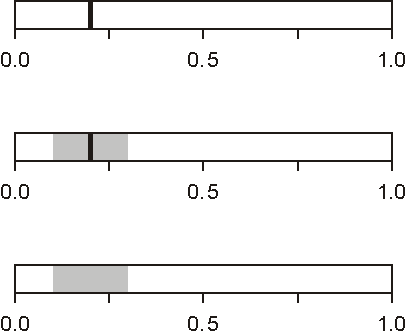
Embedded within <naivebayes> tag, this is a simple model that requires the knowledge of a-priory class probability (probability of a target class and probability of a class complementary to target class; say probability of "rains" and probability of "does not rain"), and a-priory class probability given the value of some categorical (or categorized) variable. The probabilities therefore always appear in pairs (say "0.3, 0.6"), where as a convention the probability that refers to a target class is a first one. A tag <class> is used to define unconditional priors, while conditional probabilities are expressed for each attribute and are enclosed within a tag <contingency>. To identify the variables, each conditional probability statement includes an attribute, which state an ID of a variable of interest. Here is an example of such a model: <model> <name>Naive Bayesian Model</name> <variables>Forecast;Temperature;Humidity;Windy</variables> <outcome>Probability of favorable weather to play golf</outcome> <description>A model build by naive Bayes that predicts the probability of a favorable weather for golf.</description> <naivebayes> <class>0.6, 0.4</class> <contingency> <conditional attribute="Forecast">0.6, 0.4; 0.5, 0.5; 0.66, 0.34</conditional> <conditional attribute="Temperature">0.625, 0.375; 0.5, 0.5</conditional> <conditional attribute="Humidity">0.25, 0.75; 0.83, 0.17</conditional> <conditional attribute="Windy">0.5, 0.5; 0.75, 0.25</conditional> </contingency> </naivebayes> <model> Notice that all variables that naive Bayesian model uses should be either categorical or categorized. The number of probability pairs in each definition of conditional probabilities (tag <conditional>) should exactly match match the number of values this variable can hold. While probabilities in the probability pairs are often complementary (e.g., sum to 1.0), this may in general not be so.

Logistic Regression

Logistic regression is a simple model that computes the probability using a logistic function p=1/(1+exp(-z)), where z is a linear combination of predictor variables xi, such that z=b0+b1*x1+...+bn*xn. The model is specified by coefficients in linear combination for z (bi, i=1..n; also called betas for the greek letter that is usually used for its representation). It is also evident that all predictor variables should be numerical, so a special treatment (coding) is necessary to take care for nominal variables.

An example of a simple scheme that uses a logistic regression model is triss.xml, and its "model" part is described with:

<model> <name>TRISS Model</name> <variables>GCS, SBP, RR, age, iss</variables> <outcome>TRISS Score</outcome> <logisticregression> <betas>-1.2470; 0.8941; 0.6992; 0.2775; -1.9052; -0.0768</betas> </logisticregression> </model> Notice that the model uses five variables, hence six betas are given (first one being b0, and other five associated with each of the variables). Originally, first three variables are categorical (gcs, sbp, rr; see triss.xml), but have been transformed to numerical value assigning each category its special number. Variable age is categorical, but here indices are used instead (two categories, one with index 0 and the other with 1, by default). Variable iss is numerical. Equivalent, but slightly different in treatment of GCS variable is triss_dummy.xml. Here, we use three dummy binary variables to replace 5-valued categorical variable GCS. The results (the probabilities, and GUI with this and the previous schema), however, should be just the same. As an option, logistic regression model can include information how to compute confidence intervals for a given set of variable instantiations. The mathematical background of this is given by Zupan, Porenta and Vidmar et al., here we only describe how to encode the information within the schema. Let's first show an example: <model> <name>Crush Syndrome Model</name> <variables>delay; urine; pulse</variables> <outcome>Estimated probability of severe crush syndrome:</outcome> <logisticregression> <betas>-6.4585; 1.7191; 2.4983; 0.0323</betas> <mse>0.49082</mse> <cimatrix> 0.059280, -0.005367, -0.000500; -0.005367, 0.038132, -0.000235; -0.000500, -0.000235, 0.00000719 </cimatrix> </logisticregression> </model> This is an excerpt from crush.xml, a schema that uses three variables (two categorical and one continuous). The description of logistic regression model is fairly simple, but additionally includes two elements that are used in computation of confidence intervals: these are given by <mse> and <cimatrix> tags. The matrix specified by <cimatrix> tag should be of size N times N, where N is the number of variables used in logistic regression model.

Cox Proportional Hazards Model

TBA

Probability As Derived Directly From Variable

This is the simplest model and it assumes that there is some derived variable that stores the probability that we would like to report to the user. This is the, instead of using some of the predefined model types, define the model explicitly through the use of transformations, and then report on result directly using some derived variable. A variable may define outcome probability or confidence intervals, or both. Here goes an example of the case where a variable defines the outcome probability:

<model> <name>Heat Index Model</name> <outcome>Relative Heat Index</outcome> <usevariable> <probability>heat</probability> </usevariable> </model> Notice that there should be a variable heat that should be defined and instantiated such that its values should be anything from 0.0 to 1.0 (golf_heat.xml is an example where such a model and associated transformation is used).

To include also confidence intervals, one can use: <model> <name>Heat Index Model</name> <outcome>Relative Heat Index</outcome> <usevariable> <probability>heat</probability> <confidenceintervals> <lower>heat_low</lower> <upper>heat_high</upper> </confidenceintervals> </usevariable> </model> Notice that in this case we need two more variables, one defining the lower and the other one the upper margin of confidence intervals (see golf_heat_ci.xml for a complete encoding of such model). Also, stating only confidence intervals forms a valid model: <model> <name>Heat Index Model</name> <outcome>Relative Heat Index</outcome> <usevariable> <confidenceintervals> <lower>heat_low</lower> <upper>heat_high</upper> </confidenceintervals> </usevariable> </model>

Binning

Binning can be used as an add-on for any modelling technique defined above. Remember that a model computes the probability of the target class: binning is used to re-map this probability and (optionally) associate confidence intervals. Binning is defined through definition of intervals for computed probabilities, and a value of mapped probability for each interval. Let us illustrate this through an example: <bins> <cutoffs>.1; .22; .8</cutoffs> <probabilities>.1; .2; .5; .7</probabilities> </bins> Tag <cutoffs> defines the intervals over the probability that is computed by the model. In our example there are three cut-off points, i.e. four intervals: p≤0.1, 0.1<p≤0.22, 0.22<p≤0.8, 0.8<p≤1.0 (we used p to indicate probability computed by the model). Depending on the probability returned by the model, and the interval that this probability falls-into, we can now choose from the list of probabilities and derive the final probability that will be reported to the user. Example: if the probability from, say, naive Bayesian model, is 0.15, than this will be converted to 0.2. If the probability is 0.9, than this is converted to 0.7.

Binning can also define associated confidence intervals, i.e. the final outcome would be not jus the probability, but also associated confidence intervals. In a variant of binning, confidence intervals are reported without associated mean probabilities. That is, both following binnings are valid, i.e. the one with probabilities and associated confidence intervals:

<bins> <cutoffs>.1; .22; .8</cutoffs> <probabilities>.1; .2; .5; .7</probabilities> <confidenceintervals>0.05-0.12; 0.18-0.22; 0.43-057; 0.68-0.9</confidenceintervals> </bins> and the one with confidence intervals only:

Presentation of Outcome

All models define above compute probabilities. This should be in range from 0 to 1, and should be display with 2 decimal digits (e.g., 0.23, 0.67, etc.). Logistic regression by itself, and all other methods through binning, can compute also parameters for confidence intervals. Sometimes, only confidence intervals, but not the estimated probability is known. Here are some examples how these results should be reported:

0.23
[when reporting probability only]
0.23 (0.12-0.32)
[when reporting probability and confidence intervals]
0.12-0.32
[when reporting confidence intervals only

Probabilities and confidence intervals should be, besides in text, reported also graphically. The three variants of graphs, corresponding to the tree cases mentioned above, are:

For explanation of derived probability, naive Bayes has a special way to report the influence each of variables has for the outcome. Such graph is presented in Zupan, Demsar, Kattan et al.. Only the variables which are used in naive Bayesian model appear in this graph, and their name is used for identification (label). This means that there may be cases where original variables (those that appear in the entry screen) are not present in this graph.

Logistic regression has a similar graph to help in understanding which variable contributed how to a probability of the outcome. The computation and example of this graph is reported in Zupan, Porenta, Vidmar et al.. Contrary to naive Bayes, the graph should include only original varaibles (i.e., those entered by a user). It is often the case, however, that logistic regression model includes variables that were derived from original ones instead. We may assume most general derivation model, where, say, instead of an original variable N dummy variable were used. The effects that this N dummy variables has on the outcome would then be measured and summed-up to get the effect of the original variable. The exact procedure is described in the above-mentioned paper.

Examples

golf1.xml, a simple naive Bayesian model with four variables, shows the use of pull-down, radio, and checkbox widgets to define the values of the variables. Uses for variables which are either categorical or categorized.
golf2.xml, similar to above example, but the temperature is entered as number and then categorized through the use of transformation.
golf_bins1.xml, shows example of binning
golf_bins2.xml, same as above, but binning defines only confidence intervals and does not report on expected probability.
golf_heat.xml, an example that contains two models, where the second one is based on a value of a single derived variable.
golf_heat_ci.xml, similar to above, but the second model uses two additional variables to encode confidence intervals.
triss.xml, a schema that uses a simple logistic regression model.
triss_dummy.xml, similar to above, but using additional dummy variables (the two schemas should give exactly the same results and should be used to create exactly the same GUI).
crush.xml, a schema that incorporates logistic regression model that includes data to compute confidence intervals.

Additional References

B Zupan, J Demsar, MW Kattan et al: Orange and decisions-at-hand: bridging predictive data mining and decision support, IDDM-2001. Illustrates some of the background of this endavour and shows the XML structure and GUI which were used for the previous version of DSScheme.
B Zupan, A Porenta, G Vidmar et al: Decisions at Hand: A Decision Support System on Handhelds, MedInfo-2001. This is the first paper on decision-at-hand schema, it talks about logistic regression model and its implementation on PalmOS.

Change Log

June, 2002:

multidimensional maps added in transformations,
case expression added in compute transformations.
description tag added to model
binning added to definition of models/li>
name and description tags added to definition of derived variables (this is important, since in the user's interface the value of derived should be shown in certain places, and for that we need a name that describes the variable)
derived variable can have use a tag hide to denote that the variable should not be displayed in the GUI.
special note on the use of categorical varibles in numberical expressions: their value is equal to the index of its current value from the list of values. Indices start from 0 (not 1!).
idea of having decision table as a separate model was changed; this model can be elegantly replaced through use of transformations and "usevariable" model.

Anticipated Changes and Additions

Naive Bayes can treat continuous variables directly (avoiding discretization), but there is no known standard way to present associated conditional probability curves. We will do this through splines, and description of Naive Bayesian model will be changed accordingly.
Naive Bayes can, in principle, compute confidence intervals. This has to be tested experimentally first, and once a method is stable, the description of naive Bayesian model will be augmented accordingly.
Cox proportional hazards model should be added.